Gradient Dissents

Confession 1: I’m less of a person this week. I had my appendix removed on Tuesday. It was my first surgical experience where I was anesthetized, which scared the hell out of me. Turns out that the doctor tells you to take some breaths and the next thing you know you are being woken up by a man named Nate who should really be more interested in your inebriated, albeit transcendental, commentary. 10 for 10 in terms of experiences you weren’t expecting in a week.

Confession 2: I’ve peddled myself as an R user, which I am, and R will always be my first programming language. It was my gateway to my computational and data science career, but I’m also a python user. I know, you can use both, and I frequently do, but I may program a tiny bit more in python than I do in R. Probably because of pandas, numpy and more recently tensorflow. But this post isn’t one of those stupid, click-baity, python vs. R rants; instead, it is about a common workflow of mine in which I use both together.

Collector’s Curve: A Different Measure of Diversity

Measuring diversity is one of the most fascinating parts of my research. This has been a principal theme in both of my previous posts (1, 2). A collector’s curve is a bit different than some of the other measures I have used before. The idea here is to count the unique number of items given a certain sample then increase the sample and count again. This makes the count a function of the sample size. This measure is sometimes used to measure biodiversity. I am not doing that here.

Presidential Inaugural Speeches

I thought it would be interesting to apply this concept to the number of unique words of each of the Presidents’ (of the United States) inaugural speeches as the speeches progress. In other words, I was interested at looking at the rate of unique word usage as the speech progressed and compare these across Presidential terms.

An Example

Data preparation is done in python so first we read in a handful of packages that will aid in this task.

import re # for regular expressions
import os # for operating system operations
import csv # for writing files

from nltk.corpus import inaugural
from nltk.corpus import stopwords
from nltk.stem.wordnet import WordNetLemmatizer

The fourth line is important here as that is the data, which is provided by the nltk library. It contains all of the Presidential inaugural speeches from Washington to Obama’s first term. It also comes with convenient methods for tokenizing and lemmatization.

We can take a look at Obama’s before wrapping all of these steps into one function.

obama = inaugural.words('2009-Obama.txt')
print(obama[0:9])

> ['My', 'fellow', 'citizens', ':', 'I', 'stand', 'here', 'today', 'humbled']

Thank god for the .words() method here as it tokenizes the speech for us (although writing a tokenizer isn’t too difficult 😉). Tokenization is the process of splitting words up into discrete units instead of storing them as a phrase or document. Here we can see that the tokens are the list of words of President Obama’s speech.

Next I’m going to remove stopwords (common words) and special characters. Then I will lematize each word so that I am getting each word’s root word. For example, “ran” and “run” are the same word but in different tenses. It’s not really that neat if a President (or their speech writer) just uses different grammatical variations of the same word, is it? These tasks are rather simple, just some basic list manipulation.

lemmatizer = WordNetLemmatizer()

obama_cleaned = [word.lower() for word in obama if word not in stopwords.words('english') and word.isalpha()]
obama_cleaned = [lemmatizer.lemmatize(word) for word in obama_cleaned]

Next comes the 🥖 and 🧀 (shut up. they didn’t have a butter emoji).

unique_words = []
word_len = []
counter = 0
inds = []
for word in obama_cleaned:
    inds.append(counter)
    if word not in unique_words:
        unique_words.append(word)
    word_len.append(len(unique_words))
    counter += 1

So above we start with a couple of empty lists. We will use these to store different bits of information. The first empty list, unique_words, will store each unique lemma (lemmatized word) when the iterator comes across one. The second list, word_len, will keep track of the number of unique words at the current word index. You may realize that I said sample above when discussing the curve measurement, but in this case, I can increase the sample size by one rather simply to get a complete picture of the rate change. The final list here, ids is the corresponding word index.

Alright, now I’m going to wrap this all in a nice function, add some spice to collect some metadata as we churn through these speeches and finally output a .csv.

def collect_curve_data(file):
    
    # create lemmatizer and read in corpus
    lemmatizer = WordNetLemmatizer()
    corpus = inaugural.words(file)
    
    # remove stopwords and special character and lemmatize words
    cleaned = [word.lower() for word in corpus if word not in stopwords.words('english') and word.isalpha()]
    cleaned = [lemmatizer.lemmatize(word) for word in cleaned]
    
    
    
    # the meta data
    metadata_regex = re.compile(r'(\d\d\d\d)-(\w+)\.txt')
    meta_match = metadata_regex.search(file)
    
    # find the collector's curve
    unique_words = []
    word_len = []
    counter = 0
    inds = []
    for word in cleaned:
        inds.append(counter)
        if word not in unique_words:
            unique_words.append(word)
        word_len.append(len(unique_words))
        counter += 1
    
    # gather the meta data
    year = [meta_match.group(1)] * len(word_len)
    president = [meta_match.group(2)] * len(word_len)
    vocab_size = [len(unique_words)] * len(word_len)
    
    # zip data together
    rows = zip(*[inds, word_len, vocab_size, year, president])
    
    # write output
    write_path = os.getcwd() + '/' + 'output'
    output_file = '{}/{}{}.csv'.format(write_path, meta_match.group(1), meta_match.group(2))
    
    if not os.path.exists(write_path):
        os.mkdir(write_path)
        
    
    with open(output_file, "w") as f:
        writer = csv.writer(f)
        for row in rows:
            writer.writerow(row)
            
    print('file written to: {}'.format(output_file))

Now we just iterate through all of the file ids and a collector’s curve for each Presidential inaugural speech should be written.

for file in inaugural.fileids():
    collect_curve_data(file)

Plotting the Collector’s Curves

And now I’m transition to the R portion of this post. Sorry python, none of your libraries are even worthy of standing next to ggplot2. Again, first come the packages.

library(readr)
library(dplyr)
library(purrr)
library(ggplot2)

And next we need to do some manipulation just so all of the files are easy to work with. We want them all in one data frame and to read them all from separate files, we need to use purrr’s map() and reduce() functionality, along with readr to read in the files.

files <- dir(path = "path/to/output/", pattern = "*.csv", full.names = TRUE)

data <- files %>%
  map(read_csv, col_names = c('inds', 'counts', 'vocab_size', 'year', 'president')) %>% 
  reduce(rbind)

Time for some 👏plots👏!!!! Let’s see how Obama did in 2009 in relation to all other Presidents.

obama <- filter(data, president == 'Obama')

ggplot() +
   geom_line(data = data, aes(x = inds, y = counts, group = year), colour = 'grey') +
   geom_line(data = obama, aes(x = inds, y = counts), colour = 'blue') + 
   theme_minimal() +
   ggtitle("Obama", subtitle = "2009")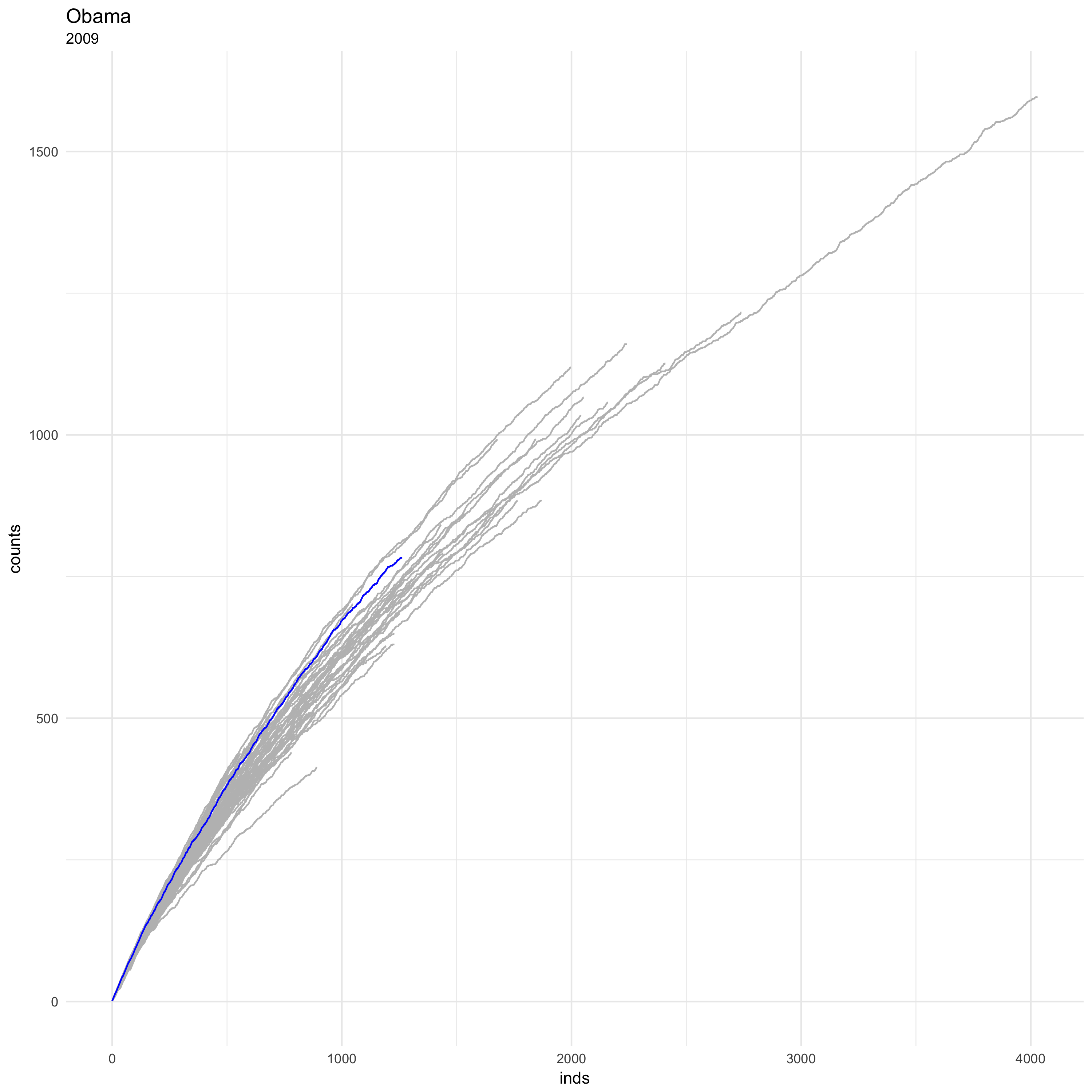

And that’s why they call it a curve. There are a couple of interesting things here. Obama uses quite a few unique words, all together it’s around 800 or so. His rate of unique word usage is also pretty high, not the highest but certainly better than a lot of the other Presidents.

But who are the rest of the curves? Let’s take a look.

full <- data %>%
 mutate(combined = paste(year, president), normalized = counts/vocab_size)

part <- data %>%
 mutate(combined = paste(year, president), normalized = counts/vocab_size) %>%
 select(-combined)
 
ggplot() +
  geom_line(data = part, aes(inds, counts, group = year), colour = 'grey', size = .5) +
  geom_line(data = full, aes(inds, counts, colour = combined)) +
  facet_wrap(~combined) + 
  theme_minimal() +
  theme(legend.position="none",
        axis.text.x = element_text(angle = 90, hjust = 1))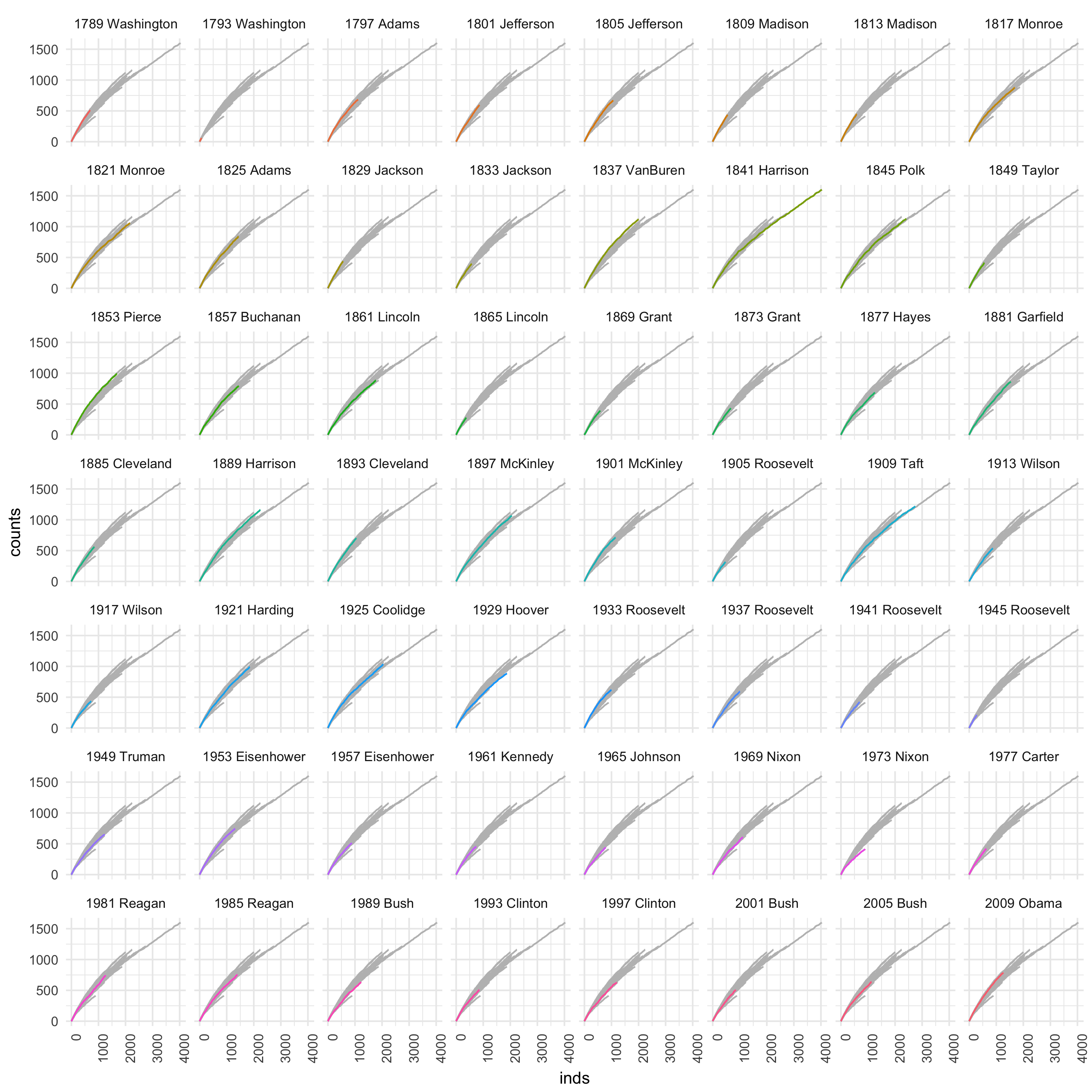 

There are a couple things to note. 1973 Washington must have had somewhere better to be. For Harrison, this was the highlight of his life (I guess that makes sense). Okay, these two observations are simply assuming that there are fewer/more unique words simply because the speeches were shorter/longer. I don’t know that for sure, but it would be easy to find out. I willing to bet on it. Pierce kept things interesting throughout his speech, at least word-wise. That can not be said for 1973 Nixon.

Wrap Things Up

Collector’s Curves are actually interesting things. Typically they are not used in such a way but they can provide some interesting insight into the diversity of different things. If you have any comments or suggestions, please feel free to leave them! I will touch on collector’s curves again as it pertains to the linguistic diversity of a region.