Gradient Dissents

There are very few recent packages that I can say shaved a month off of my dissertation work, particularly in a language like R where there are 3,000,000 ways to do the same thing. But tidycensus, my hat’s off to you 👏👏👏! If you need Census data (or not) I strongly urge you to check out Kyle Walker’s tidycnesus.

Diversity is a difficult concept. It might be even more difficult to assess simply because there are several ways to measure it. I’m not going to discuss all of these measures nor am I going to really go over definitions in this post, but if you are interested in how to assess diversity I recommend checking out Scott Page’s Diversity and Complexity. Instead, I’m going to dive into the world of assessing the racial diversity¹ of cities using data gathered from the American Community Survey, but first a problem:

Imagine you are tasked with assessing the racial diversity of a city block. Let’s make it simple, we only need to assess the diversity of that city block for those individuals that live there. Forget about considering the people who just work or pass through (admittedly, this is important but adds complexity). How do you assess the “diversity” of the city block? Count the number of racial categories? Perhaps, but is a place that has 100,000 white individuals, 1 black individual and 1 Native Hawaiian more diverse than a location with 5,000 white individuals and 5,000 black individuals? Furthermore, even the smallest of towns will have a similar number of racial categories as some of the largest cities.

What I want is a measure that considers both the number of unique categories along with the evenness of those categories. Sounds like an entropy measure, right? Well, in ecology, biologists are often interested in measuring the biodiversity of an ecosystem. To do so they calculate what is known as a Shannon Index $H$.

$$H = -\sum_{i=1}^R p_i\ln p_i$$

$R$ here is the total number of racial categories and $p_i$ is the proportion of $R$ made up by the $i$^th category.

And now for data! The Census’ data portal is the closest thing to hell on the internet after r/TheDonald, which is why I am eternally indebted to Kyle Walker and the godsend that is tidycensus. I encourage you to follow along so if you haven’t already obtained a free api key from the Census API, go here². We are going to need a handful of packages to get started.

library(tidyverse)  
library(tidycensus)
library(sf) 
library(vegan)
library(viridis)
library(tigris)
library(ggthemes)

options(tigris_class = "sf")
options(tigris_use_cache = TRUE)

Now we need a city. How about Cincinnati? I have no affiliation with Cincinnati but everyone seems to use New York for these types of tasks so why not shake things up? So to get started we need a list of the counties that make up the Cincinnati metro area along with the ACS codes pertaining to racial categories in the 2015 American Community Survey. The ACS provides estimates and for greater reliability we are using Census tracts. I am first going to create a vector of counties in the following format "StateAbberviationCountyName". For example, Boone county, Missouri would become "MOBoone". Then we need a vector of ACS codes that we want to collect.

places <- c(
  'OH,Brown', 'OH,Butler', 'OH,Clermont', 'OH,Clinton', 'OH,Hamilton', 'OH,Warren', 'KY,Boone', 'KY,Bracken',
  'KY,Campbell', 'KY,Gallatin', 'KY,Grant', 'KY,Kenton','KY,Mason', 'KY,Pendleton', 'IN,Dearborn', 'IN,Franklin', 
  'IN,Ohio')

racevars <- c('B02001_002E', 'B02001_003E', 'B02001_004E', 'B02001_005E', 'B02001_006E',
              'B02001_007E', 'B02001_008E', 'B02001_009E', 'B02001_010E')

Now we want to feed these into the get_acs function which will return the estimates from each tract, but first we have to wrap that in purrr’s map capabilities along with some string manipulation provided by stringr.

pop <- reduce(
  map(places, function(x) {
    get_acs(geography = "tract", variables = racevars, 
            state = str_split(x ,pattern = ',')[[1]][1],county = str_split(x,pattern = ',')[[1]][2])
  }), 
  rbind
)

geographies <- reduce(
  map(places, function(x) {
    get_acs(geography = "tract",  variables = 'B01003_001',
            state = str_split(x ,pattern = ',')[[1]][1],county = str_split(x,pattern = ',')[[1]][2] ,
            geometry = TRUE, cb = FALSE)
  }), 
  rbind
)

water <- reduce(
  map(places, function(x){
    area_water(str_split(x ,pattern = ',')[[1]][1], str_split(x,pattern = ',')[[1]][2], 
               class = "sf")
  }),
  rbind
)

We are going to perform a variant of this 3 times in order to collect the estimates, the shapefiles of those regions, and the water polygons for better map detail. You may wonder why we are collecting the shapefiles separate from the estimates. Well, we have to perform an aggregation and aggregations don’t work very well on Multipolygon attributes. Eventually, we will join these all together. Below we will borrow a Kyle Walker function to remove water areas from geographies.

st_erase <- function(x, y) {
  st_difference(x, st_union(st_combine(y)))
}

cin_erase <- st_erase(geographies, water)

And finally, we use the vegan package to calculate Shannon over the race variables that we collected in the pop dataframe. We want to calculate it for each Census tract to get an idea of where are the more racially diverse areas of the city.

# calculate shannon on race and map it!
pop %>% 
  group_by(GEOID) %>%
  summarise(diversity = diversity(estimate)) %>%
  left_join(cin_erase) %>% 
  ggplot(aes(fill = diversity, color = diversity)) +
    geom_sf() + 
    scale_fill_viridis() + 
    scale_color_viridis() + 
    theme_map()+
    theme(panel.grid.major = element_line(colour = "white"))

This produces the following map:

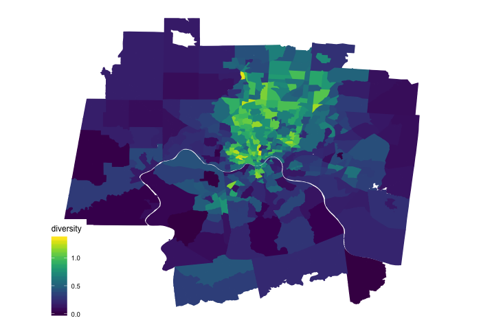
There are a couple things to note about this graph. The first is that the tracts are trimmed based off of geographical center of the city that I didn’t show within the code (this will come in future posts). Secondly, the center of the city tends to be more diverse than the margins. In other words, the suburbs tend to be a less racially diverse than the center of the city.

In future posts, I will continue down this path of measuring diversity and, more interestingly, why this is important to understanding other characteristics of a city.

Links that helped along the way

1. Loading and analysing spatial data with the sf package by Pierre Roudier
2. retrieve coordinate reference system from object
3. Manipulating Simple Feature Geometries

Footnotes

1: Keep in mind that “race” here isn’t meant as a biological category to classify individuals into groups. Instead, it is simply a Census categorization of individuals and how they identify themselves.

2: This page is straight out of the 90s but it works.