Gradient Dissents

This was one of those moments where my Googling ability failed me. For learning purposes, this is great, but in terms of time, well I’m never getting those couple of days in February back. So this is a story about how I thought I solved a problem that had yet to be solved. This is also a story about how I was stupid to think that I was the first to solve a problem that must be fairly common.

I’m interested in cities and their people, and city metropolitan areas often span multiple counties, however, not all counties are equal particularly in terms of area. Seriously, look up San Bernardino county, California and see how many New England states you can fit inside it. Well, the problem is that you are often not interested in all of the super-geographies during an analysis. Instead, you are interested in some sub-geographies that make up a certain radius around a coordinate. This was my issue and this post is going to walk you through two different solutions: one out of naïveté and the other a bit more researched.

Kansas City is the perfect candidate to test subsetting around a coordinate. Its metropolitan area spans 9 counties and 2 states (the majority in Missouri and some in Kansas). Just to be exhaustive, I will be collecting on a 15 county area. It also happens to be my place of birth and where I spent the majority of the first 18 years of my life. I will be using tidycensus to gather the Census tracts for each of these counties along with the 2015 American Community Survey estimates on the proportion of Black Americans living in each tract. Take a look at my previous post for a more detailed explanation of using tidycensus to collect ACS data. First we will load in our packages and then gather our data.

library(tidyverse)  
library(tidycensus)
library(sf) 
library(vegan)
library(viridis)
library(tigris)
library(ggthemes)

options(tigris_class = "sf")
options(tigris_use_cache = TRUE)

# ACS 2015 race variable codes

racevars = c('B02001_001E', 'B02001_003E')

# Counties 

places <- c('MO,Clay', 'MO,Jackson', 'MO,Platte', 'MO,Cass', 'MO,Lafayette',
            'MO,Ray', 'MO,Clinton', 'MO,Bates', 'MO,Caldwell', 'KS,Johnson',
            'KS,Wyandotte', 'KS,Leavenworth', 'KS,Miami', 'KS,Linn', 'KS,Franklin')

# Collect the variables

pop <- reduce(
  map(places, function(x) {
    get_acs(geography = "tract", variables = racevars, 
            state = str_split(x ,pattern = ',')[[1]][1],county = str_split(x,pattern = ',')[[1]][2])
  }), 
  rbind
)

# Collect the simple features for mapping

geographies <- reduce(
  map(places, function(x) {
    get_acs(geography = "tract",  variables = "B01003_001",
            state = str_split(x ,pattern = ',')[[1]][1],county = str_split(x,pattern = ',')[[1]][2] ,
            geometry = TRUE)
  }), 
  rbind
)

Then I have to do some pre-processing. B02001_001E is the variable for the total number of people estimate for the selected geography and B02001_003E is the estimate of African Americans within a geography. I want a proportion instead of raw count so I have to convert the current pop data frame into wide format. Wide format allows me to use mutate in order to calculate a proportion. I then join this back to the geographic simple features data frame geographies so that we can visualize the proportion graphically.

pop %<>%
  select(-moe) %>%
  spread(variable, estimate) %>%
  group_by(GEOID) %>%
  mutate(aa = (B02001_003/B02001_001)) %>%
  ungroup()

kc <- geographies %>%
  left_join(pop, by = 'GEOID') 

Let’s go ahead and visualize what we have here.

kc %>%
  ggplot(aes(fill = aa)) + 
  geom_sf( colour = '#ffffff', size = 0.1) + 
  scale_fill_viridis(option = "inferno", direction = -1) +
  labs(title = "Kansas City's Black American Population",
       subtitle = "Proportion by Census Tract" ,
       caption = 'Data: 2015 American Community Survey')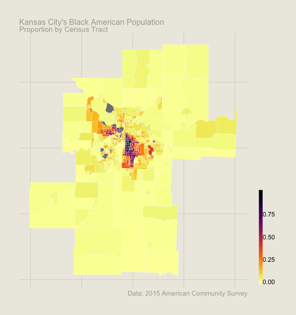

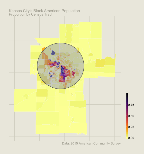
Oh my! I’m more interested in the city center and the surrounding suburbs, not really those who are in the exoburbs. Let’s try those within a 40 kilometer radius of the center of Kansas City, MO. Any tract that is captured in this circled area below is permitted. Everyone else, well thanks for playing and perhaps next time.

Before I dive into my solutions, I want to extend my highest praise for the sf package. It is written with usability in mind so if you are working with simple features, checkout sf if you haven’t already. It also integrates with the dplyr pipe (%>%) so HOLLA 🙌!!!

Attempt 1: Lessons in Naïveté

I felt okay about this method until I came across a much cleaner and more elegant way of achieving the stated goal but I am also a believer in working through problems on your own and configuring your own solutions, even if it means embarrassing yourself when you put it on the web.

My algorithm is as follows. First, declare a center point for the city of Kansas City. This was as difficult as Googling ‘Kansas City coordinates’. Then, I would write a function that can be applied row-wise to a data frame to calculate the distance between the row’s simple feature and the geographic center of Kansas City. I run this function over the kc data frame created above. Then I simply subset for those rows within 40 km and then plot. Voilà!

# Kansas City Coordinates to calculate distance from 
kc_center <- st_sfc(st_point(c(-94.5786 ,  39.0997)))
kc_center = st_sf(geom = kc_center)
st_crs(kc_center) = 4326

# function to calculate the closet point of each census tract
find_distance <- function(row, coord){
  row %>% 
    st_cast('POINT') %>%
    st_transform(crs = 32119) %>%
    st_distance(st_transform(coord, crs = 32119)) %>%
    min()
}

kc_sub <- kc %>% 
  by_row(.collate = "cols", function(row){
    row %>% 
      st_cast('POINT') %>%
      st_transform(crs = 32119) %>%
      st_distance(st_transform(kc_center, crs = 32119)) %>%
      min() %>% 
      unlist() 
  })

# subset and plot
kc_sub %>% 
  filter(.out <= 40000) %>%
  ggplot(aes(fill = aa)) + 
  geom_sf( colour = '#ffffff', size = 0.1) + 
  scale_fill_viridis(option = "inferno", direction = -1) +
  labs(title = "Kansas City's Black American Population",
       subtitle = "Proportion by Census Tract" ,
       caption = 'Data: 2015 American Community Survey')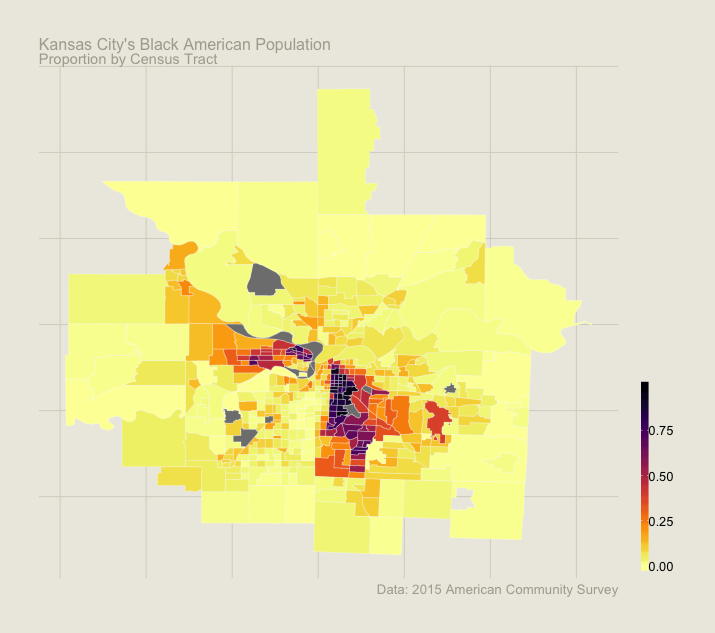

This worked but there was something that didn’t sit well with me about all of this code. It was too much for something that had to be a lot more common. So for the second time in two days I found myself checking the interwebs for those who have surely done this task.

Attempt 2: Lessons in Humility

This method requires me to transform the default Coordinate Reference System (CRS) for the kc data frame but after you get through that, the following functions are rather intuitive. It requires you specifying the point coordinates of the center of the city, similar to the first solution, but then creating a buffer of x distance around this point. From there it is as simple as finding the intersection of this buffer and the kc data frame and then subsetting the data based off of this intersection.

# convert crs 

kc_sf <- st_sf(kc)
new_proj <- "+proj=aea +lat_1=29.5 +lat_2=45.5 +lat_0=37.5 +lon_0=-96 +x_0=0 +y_0=0 +ellps=GRS80 +units=m +no_defs"
kc_sf <- st_transform(kc_sf, st_crs(new_proj))

# create buffer of 40 km
kc_ctr_sfc <- st_sfc(st_point(c(-94.5786 ,  39.0997)), crs = 4326)
kc_ctr_aea_sf <- st_transform(kc_ctr_sfc, st_crs(kc_sf))
kc_buf_sf <- st_buffer(kc_ctr_aea_sf, 40000)

# find intersection and subset
kc_buf_intersects <- st_intersects(kc_buf_sf, kc_sf)
kc_sel_sf <- kc_sf[unlist(kc_buf_intersects),]

# plot
kc_sel_sf %>%
  st_transform( crs = 4326) %>%
  ggplot()+
  geom_sf(aes(fill = aa), colour = '#ffffff', size = 0.1) + 
  scale_fill_viridis(option = "inferno", direction = -1) +
  labs(title = "Kansas City's Black American Population",
       subtitle = "Proportion by Census Tract" ,
       caption = 'Data: 2015 American Community Survey')

And this renders…

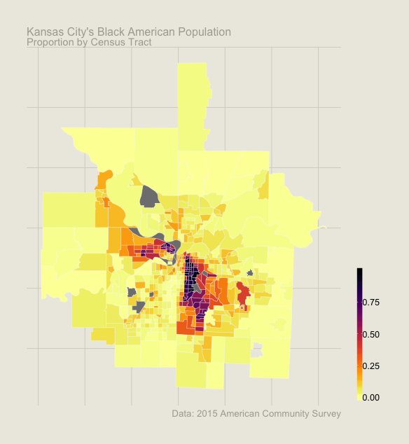
Okay, the good news is that my original solution and the second solution render the same map. That’s a good sign that they are working. The other (neutral) news is that I want to zoom in a bit more. Let’s say 20 kilometers from the city center. Since this task was becoming somewhat repetitive I thought a function could really help out…

subset_map <- function(df, long, lat, dist = 40000){
  # Change CRS for buffer
  df_sf = sf::st_sf(df)
  new_proj = "+proj=aea +lat_1=29.5 +lat_2=45.5 +lat_0=37.5 +lon_0=-96 +x_0=0 +y_0=0 +ellps=GRS80 +units=m +no_defs"
  df_sf = sf::st_transform(df_sf, sf::st_crs(new_proj))
  
  # Prepare buffer around center point
  cntr_pnt <- sf::st_sfc(sf::st_point(c(long ,  lat)), crs = 4326)
  cntr_aea_sf <- sf::st_transform(cntr_pnt, sf::st_crs(df_sf))
  buff <- sf::st_buffer(cntr_aea_sf, dist)
  
  # Subset original data
  intersection <- sf::st_intersects(buff, df_sf)
  subset <- df_sf[unlist(intersection),]
  
  subset
  
}

This made things a lot easier. Oh and just for the hell of it I’m going to add a layer of highways, which can be found here.

highways <- st_read('~/Downloads/highway_system/highway_system.shp')

subset_map(kc_sub, -94.5786, 39.0997, dist = 20000) %>%
  ggplot()+
  geom_sf(aes(fill = aa), colour = '#ffffff', size = 0.1) + 
  geom_sf(data = highways, color = '#d1d0cf') +
  theme_mapper()+
  scale_fill_viridis(option = "inferno", direction = -1) +
  labs(title = "Kansas City's Black American Population",
       subtitle = "Proportion by Census Tract" ,
       caption = 'Data: 2015 American Community Survey')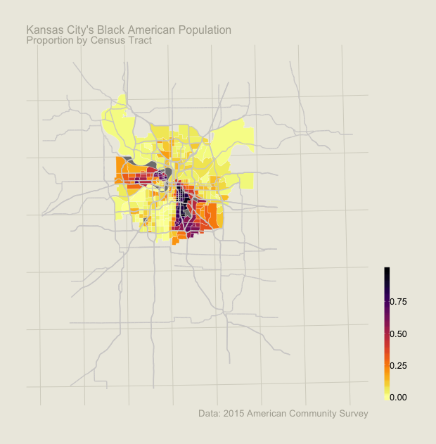

Whoops! The highways layer would look better if it were also subset.

highway_sub <- subset_map(highways, -94.5786, 39.0997, dist = 20000)

subset_map(kc_sub, -94.5786, 39.0997, dist = 20000) %>%
  ggplot()+
  geom_sf(aes(fill = aa), colour = '#ffffff', size = 0.1) + 
  geom_sf(data = highway_sub, color = '#d1d0cf') +
  theme_mapper()+
  scale_fill_viridis(option = "inferno", direction = -1) +
  labs(title = "Kansas City's Black American Population",
       subtitle = "Proportion by Census Tract" ,
       caption = 'Data: 2015 American Community Survey')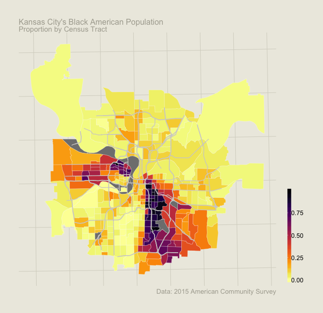

And there we have it! And once again…

Links that have helped me along the way…

• Operations with Spatial Vector Data in R by Claudia A Engel
• Introduction to spatial site-suitability analysis in R by Ken Steif